Vignette (Example Data)
Instructions and files provided will allow the user to walk through an automated and a manual run of Breathe Easy. The larger files, i.e., .txt files and .adicht files, are hosted on our Zenodo account due to their size.
The output for the automated run and manual run are slightly different. We have provided the exact configuration files for both runs that produce the output displayed in each section. Once you are comfortable with the STAGG settings subGUI, explore a bit to see the other options for displaying your data.
Ex. LabChart Exporting
Example LabChart files (.adicht format) are provided to allow users to practice the conversion process and batch exporting of DataPad selections.
Download the dataset containing the LabChart files (doi: 10.5281/zenodo.7144692) from Zenodo.
Follow detailed user guide to batch export .adicht files to .txt format.
Follow instructions to batch export DataPad selections from LabChart files into .txt format.
Ex. Automated Run
Example .txt files (already exported to required format) are provided on our Zenodo site. Internal links in the below instructions will take you to pages with more detailed instructions on completing each of the steps below.
Download the Zenodo dataset containing the .txt formatted LabChart file exports for the vignette dataset (doi: 10.5281/zenodo.7120978) at Zenodo’s website.
Initialize SASSI by selecting input files (the downloaded .txt files) and your desired output folder.
Load the metadata using the below provided metadata.csv file. No changes are needed, unless you want to explore options. However, it should be noted that any changes to the below file made within the subGUI or in the file itself will not guarantee a successful run.
Load provided automated settings.
-
Your JSON file output from the SASSI run should automatically populate the input for STAGG. If this does not happen for some reason, then please follow the instructions provided here to select the appropriate JSON files.
Load provided settings for STAGG run. You will need to select all 3 settings files when choosing the option to
Select file.Note
It should be noted that many changes and options can be explored in the STAGG settings subGUI. It is imperative to note, however, that changes made by the user may not result in a successful run. So, if this is your first time using Breathe Easy, we recommend not making any changes, bur rather noting the selections made.
Once the STAGG settings are made, select your desired file type output (.jpeg or .svg) and run STAGG.
For help understanding the outputs for STAGG or SASSI, see the linked sections of this manual.
Automated Run Output
This is what your SASSI and STAGG output folders should look like for the automated run outlined above.
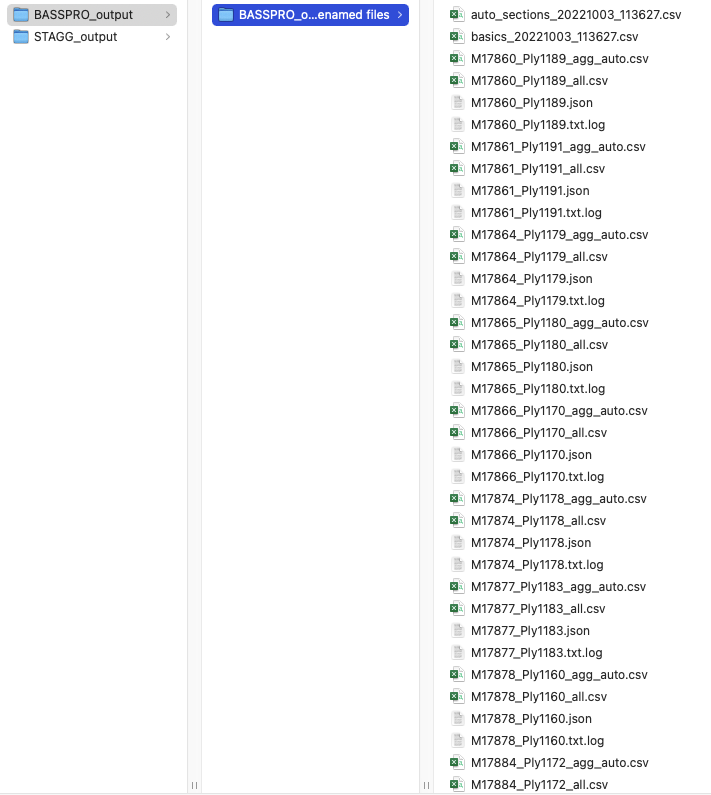
Screenshot of the SASSI output folder for automated run instructions in vignette.
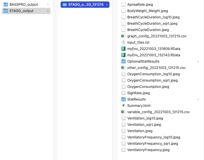
Screenshot of the STAGG output folder for automated run instructions in vignette.
Some of the figures generated in this run are below.
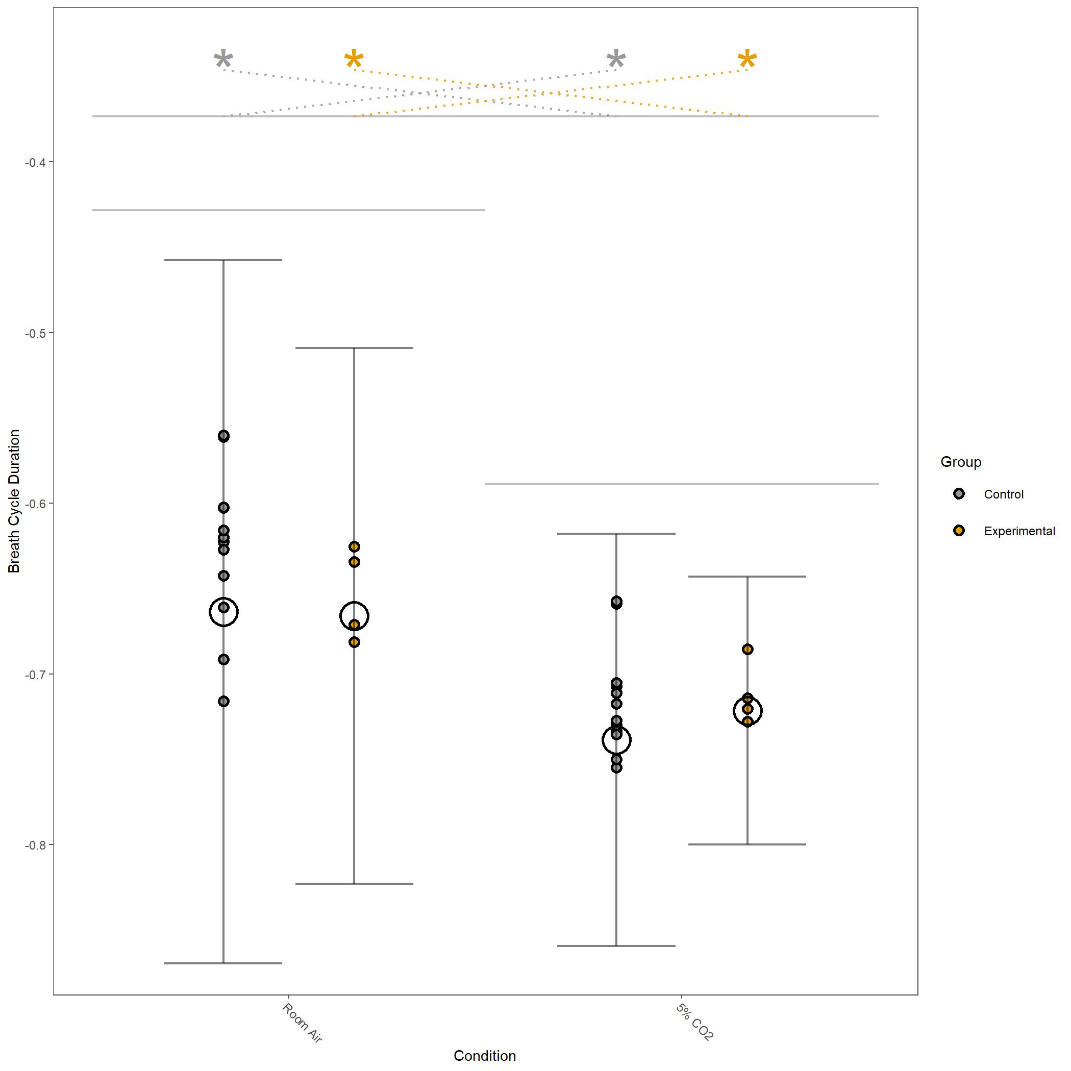
Log10 transformed Breathe Cycle Duration for vignette dataset.
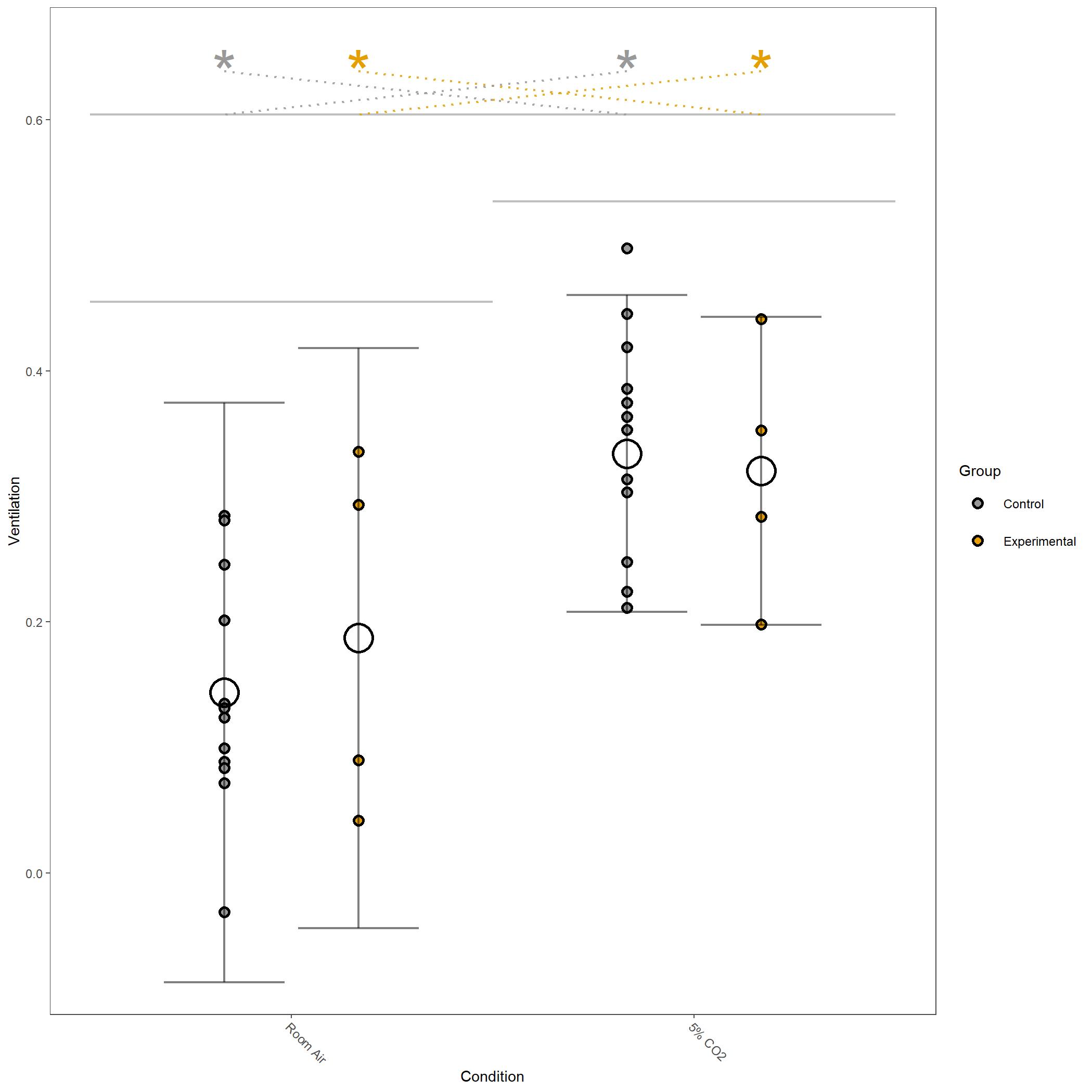
Log10 transformed Ventilation for vignette dataset.
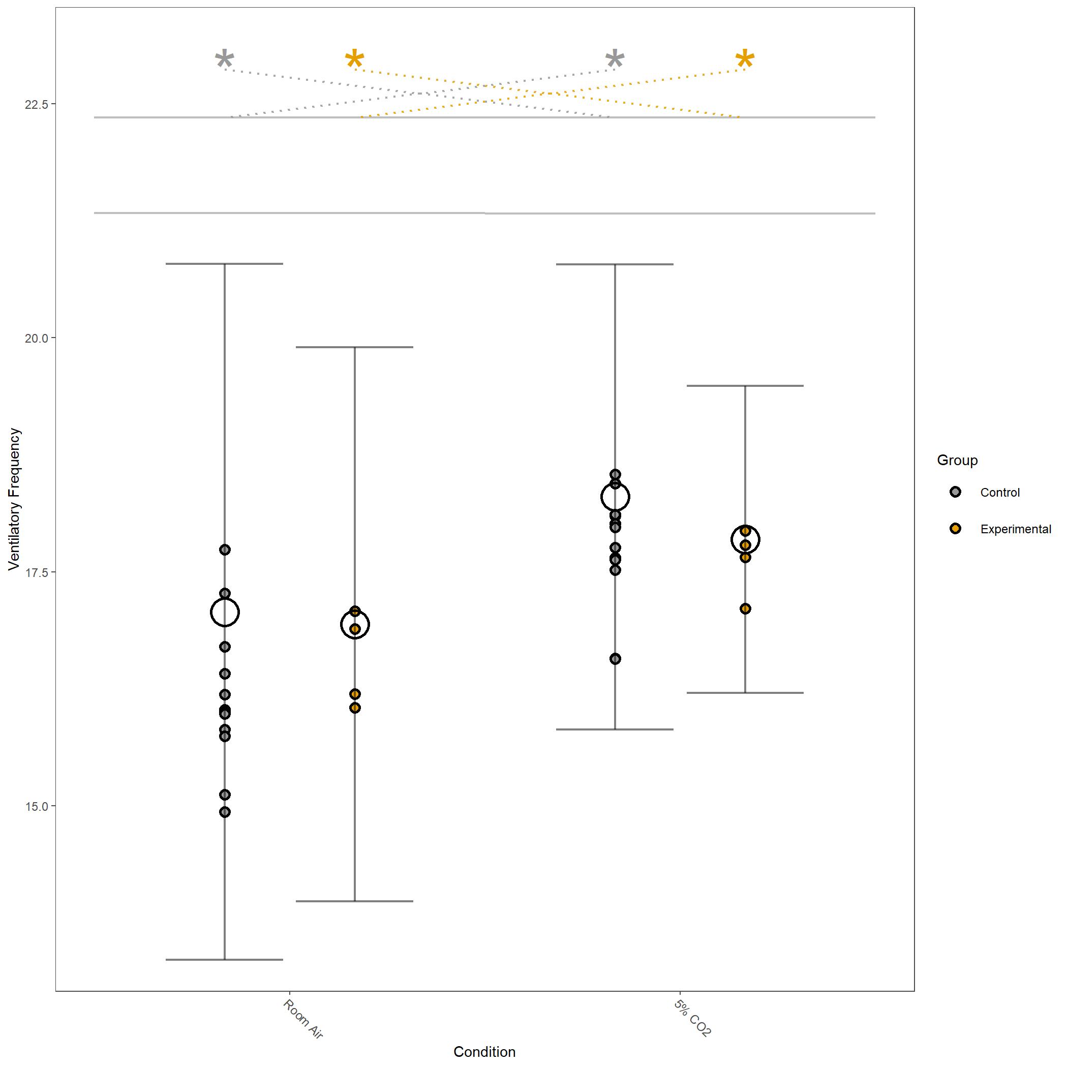
Square root transformed Ventilatory Frequency for vignette dataset.
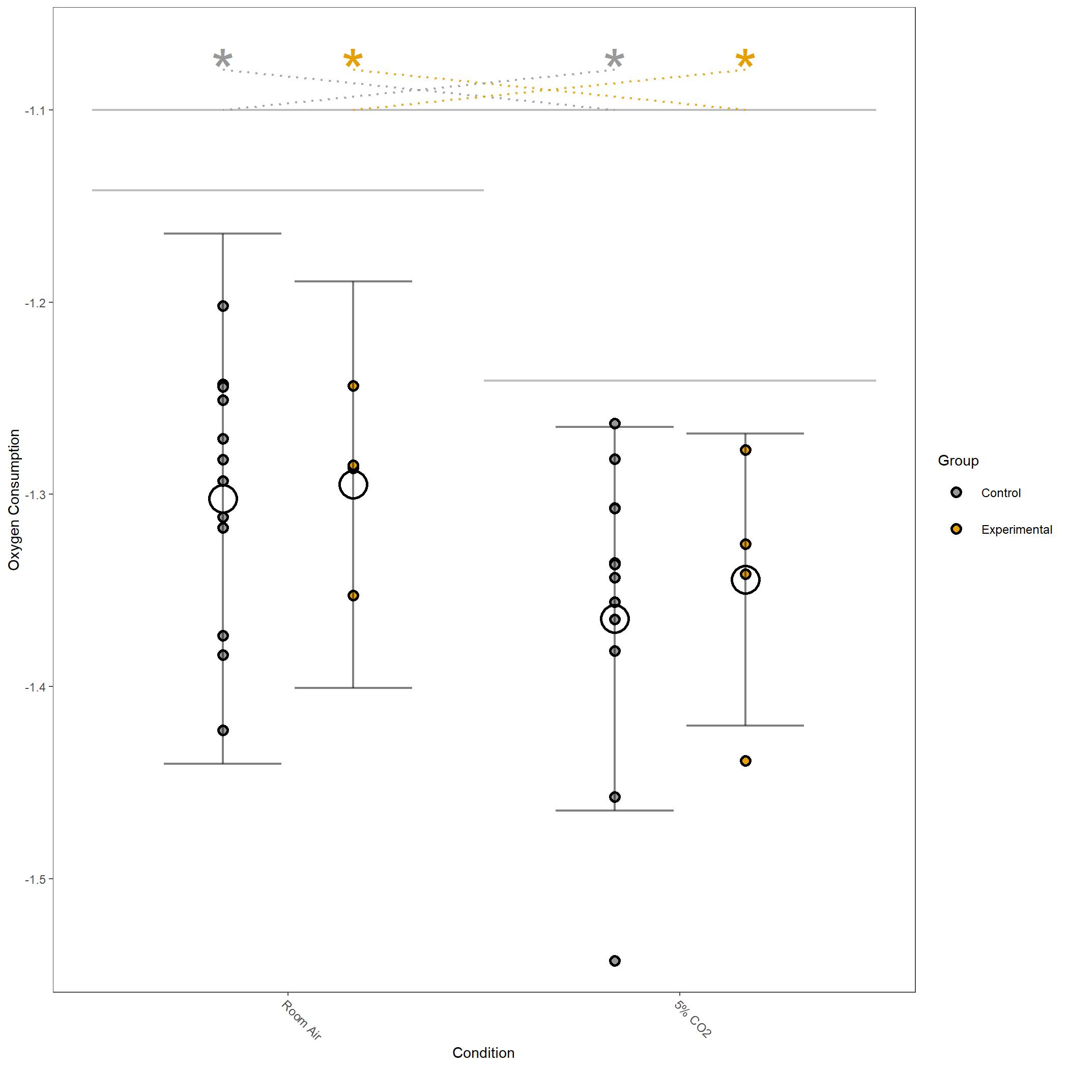
Log10 transformed Oxygen Consumption for vignette dataset.
Within the StatResults folder are the residual and QQ plots for all transformations. These are used to determine
the most appropriate transformation for each variable. To demonstrate the use of these, we’ve hightlight the selection
of the appropriate transformation of Breath Cycle Duration below where the raw values, log10 transformed, and
square root transformed QQ and residual plots are shown. We chose log10 transformed becuase the QQ plot showed the most
linear-like distribution and the residual plot was least skewed for that transformation of the data. This is the process
that was completed for each of the variables above to select the appropriate statistical outcomes.
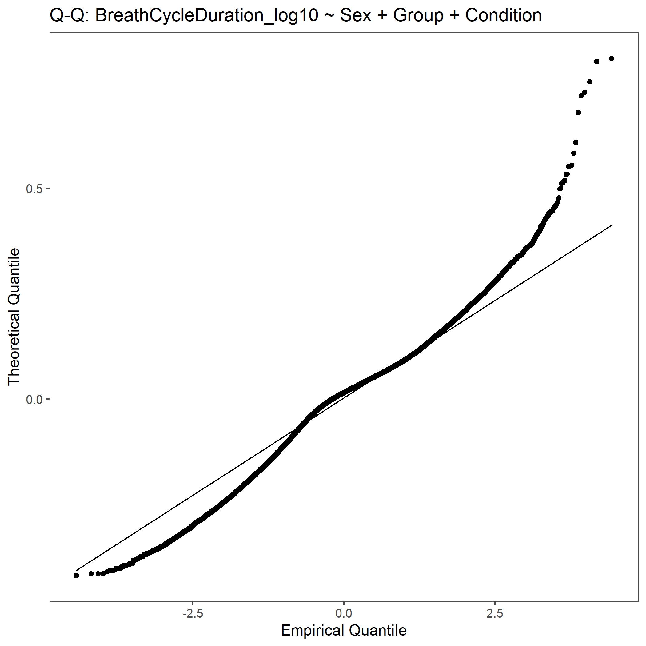
QQ plot for Breath Cycle Duration with log10 transformed data.
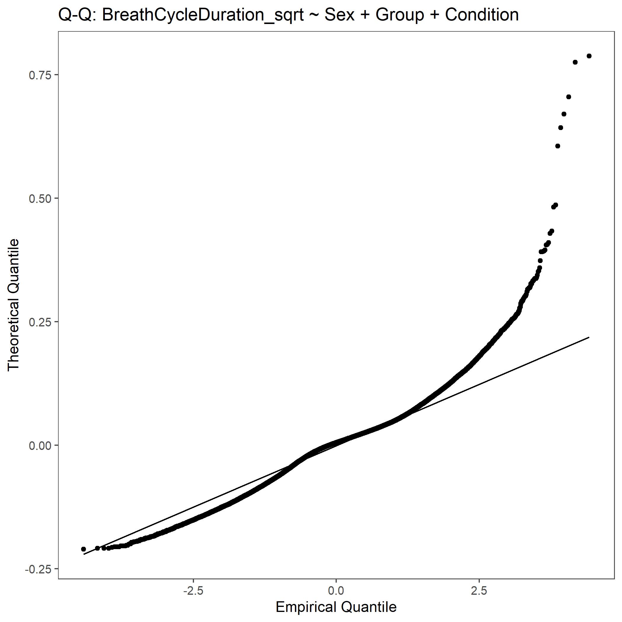
QQ plot for Breath Cycle Duration with square root transformed data.
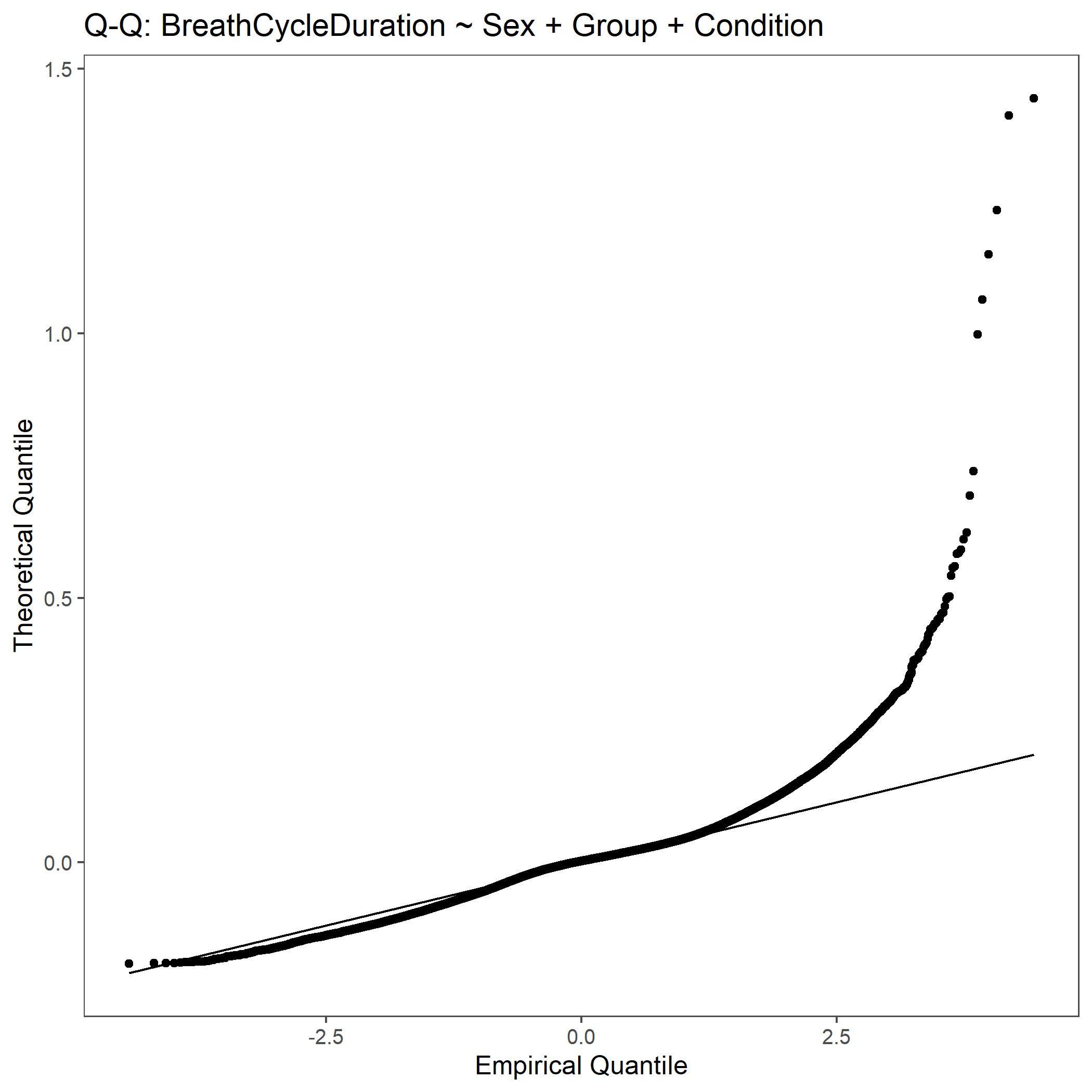
QQ plot for Breath Cycle Duration with non-transformed, raw data.
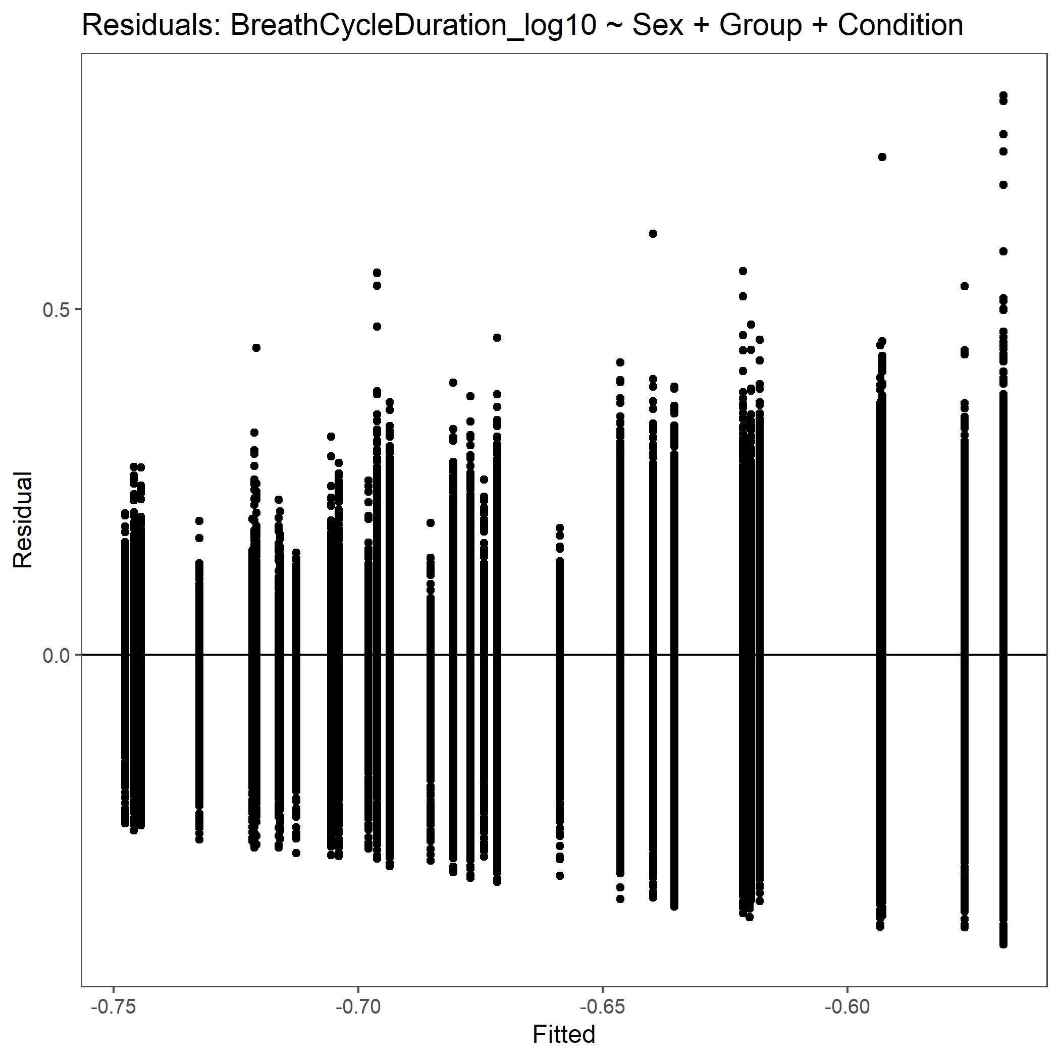
Residual plot for Breath Cycle Duration with log10 transformed data.
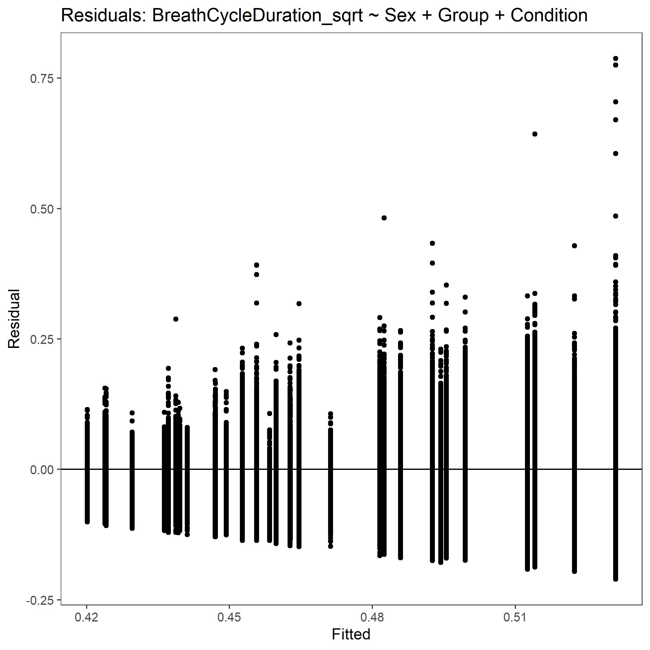
Residual plot for Breath Cycle Duration with square root transformed data.
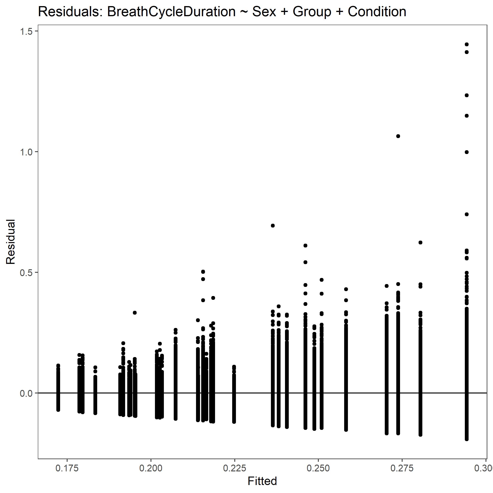
Residual plot for Breath Cycle Duration with non-transformed, raw data.
Ex. Manual Run
Example .txt files (already exported to required format) are provided on our Zenodo site. Internal links in the below instructions will take you to pages with more detailed instructions on completing each of the steps below.
Download the dataset containing .txt formatted LabChart file exports for the vignette dataset (doi: 10.5281/zenodo.7120978) at Zenodo’s website.
Initialize SASSI by selecting input files (the downloaded .txt files) and your desired output folder.
Load the metadata using the below provided metadata.csv file. No changes are needed, unless you want to explore options. However, it should be noted that any changes to the below file made within the subGUI or in the file itself will not guarantee a successful run.
Load provided manual settings.
Note
If you want to practice making the manual settings file, we have provided the DataPad exports for this dataset on Zenodo. (doi: 10.5281/zenodo.7120968). Use these files with a 5% CO2 experimental design to generate the manual settings provided here. See full manual settings instructions for more information.
-
Your JSON file output from the SASSI run should automatically populate the input for STAGG. If this does not happen for some reason, then please follow the instructions provided here to select the appropriate JSON files.
Load provided settings for STAGG run. You will need to select all 3 settings files when choosing the option to
Select file.Note
It should be noted that many changes and options can be explored in the STAGG settings subGUI. It is imperative to note, however, that changes made by the user may not result in a successful run. So, if this is your first time using Breathe Easy, we recommend not making any changes, but rather noting the selections made.
Once the STAGG settings are made, select your desired file type output (.jpeg or .svg) and run STAGG.
For help understanding the outputs for STAGG or SASSI, see the linked sections of this manual.
Manual Run Output
This is what your SASSI and STAGG output folders should look like for the automated run outlined above.
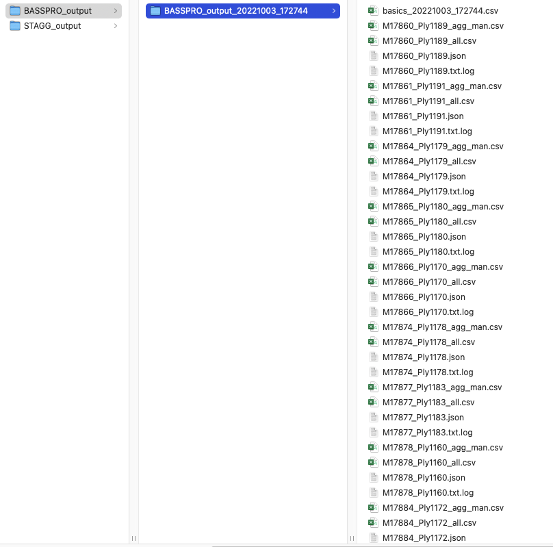
Screenshot of the SASSI output folder for manual run instructions in vignette.
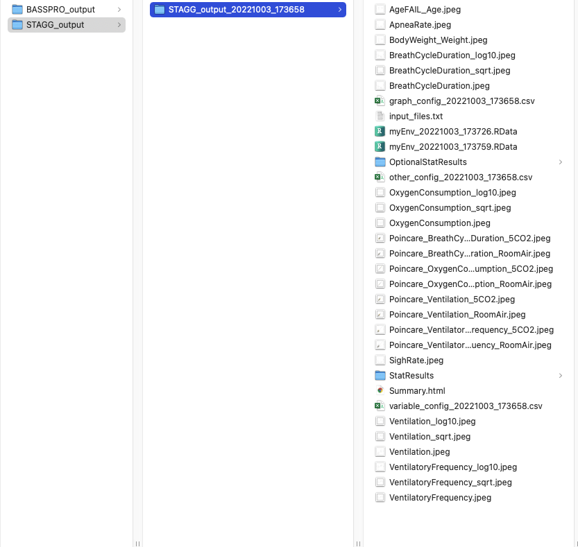
Screenshot of the STAGG output folder for manual run instructions in vignette.
For this example we’ve included body weight as an example of metadata figures.
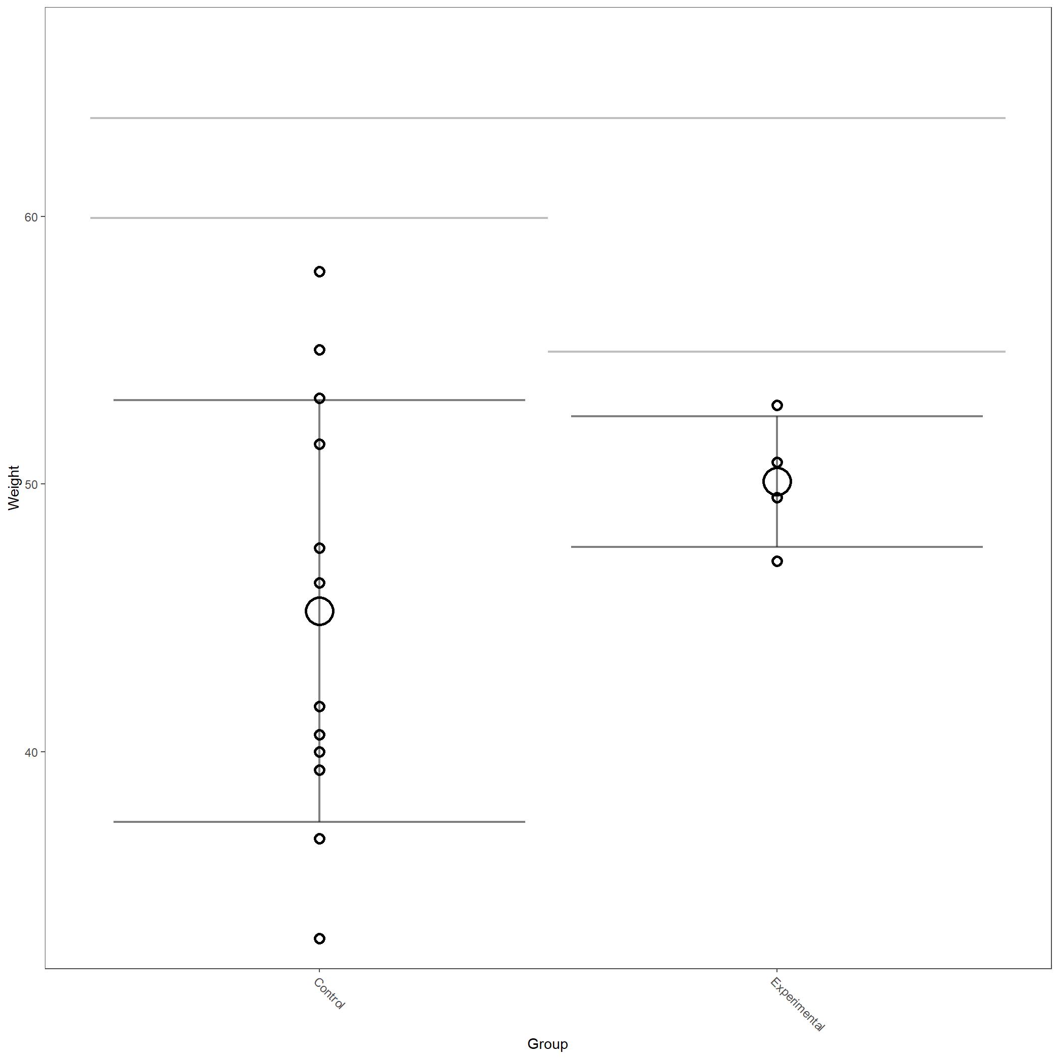
Body weight of animals included in manual Breathe Easy vignette.
Some of the figures for respiratory variables generated in this run are below.
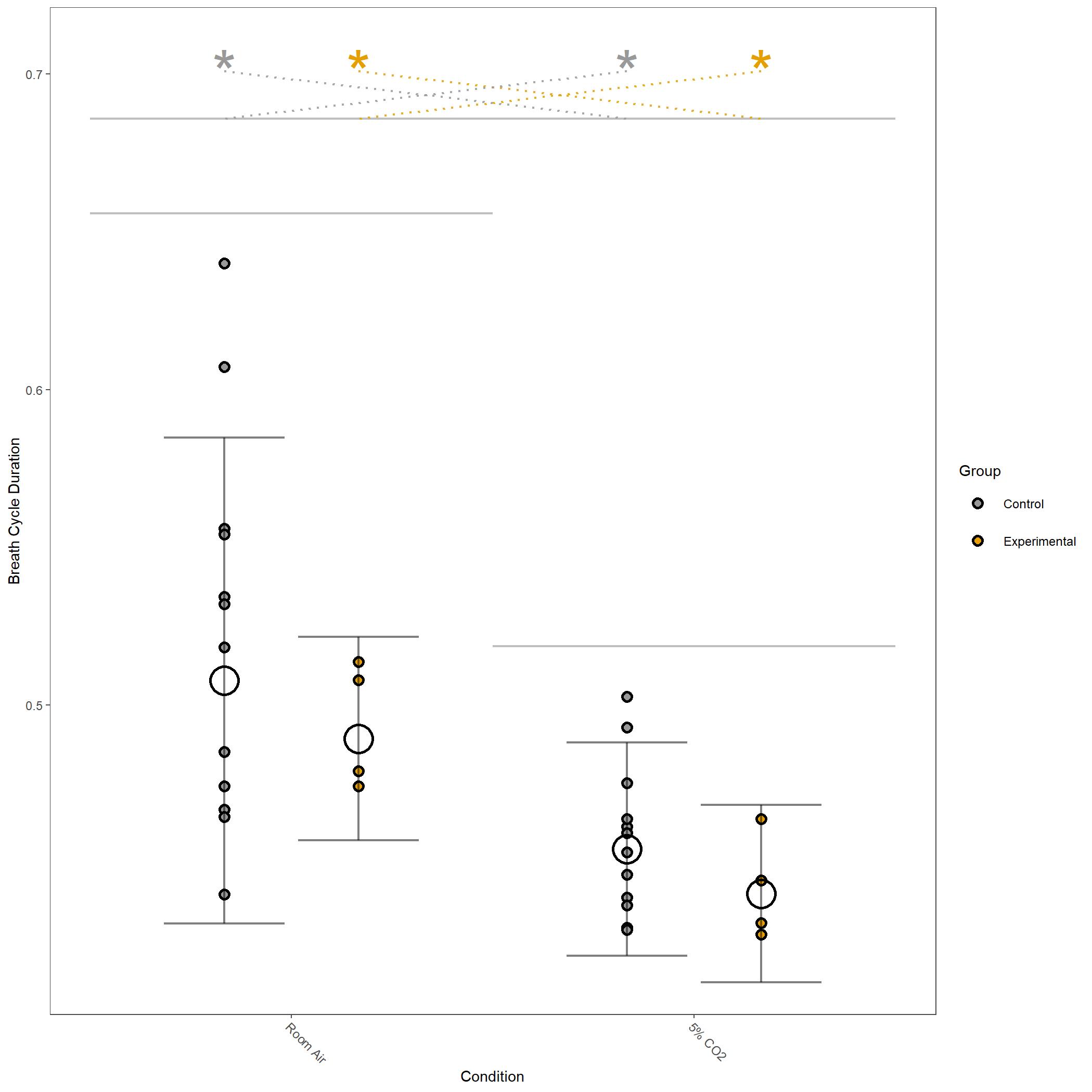
Square root transformed Breathe Cycle Duration for vignette dataset.
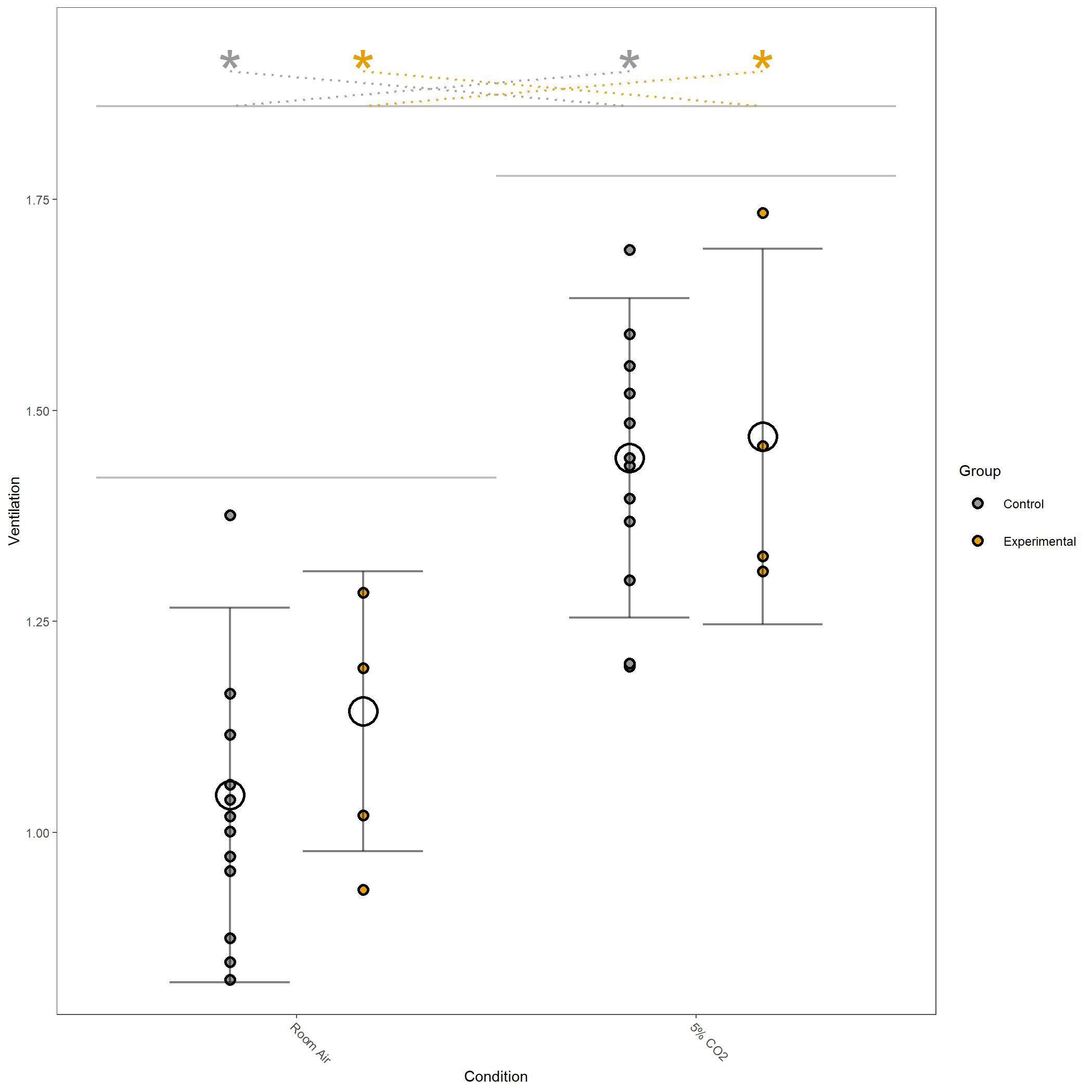
Square root transformed Ventilation for vignette dataset.
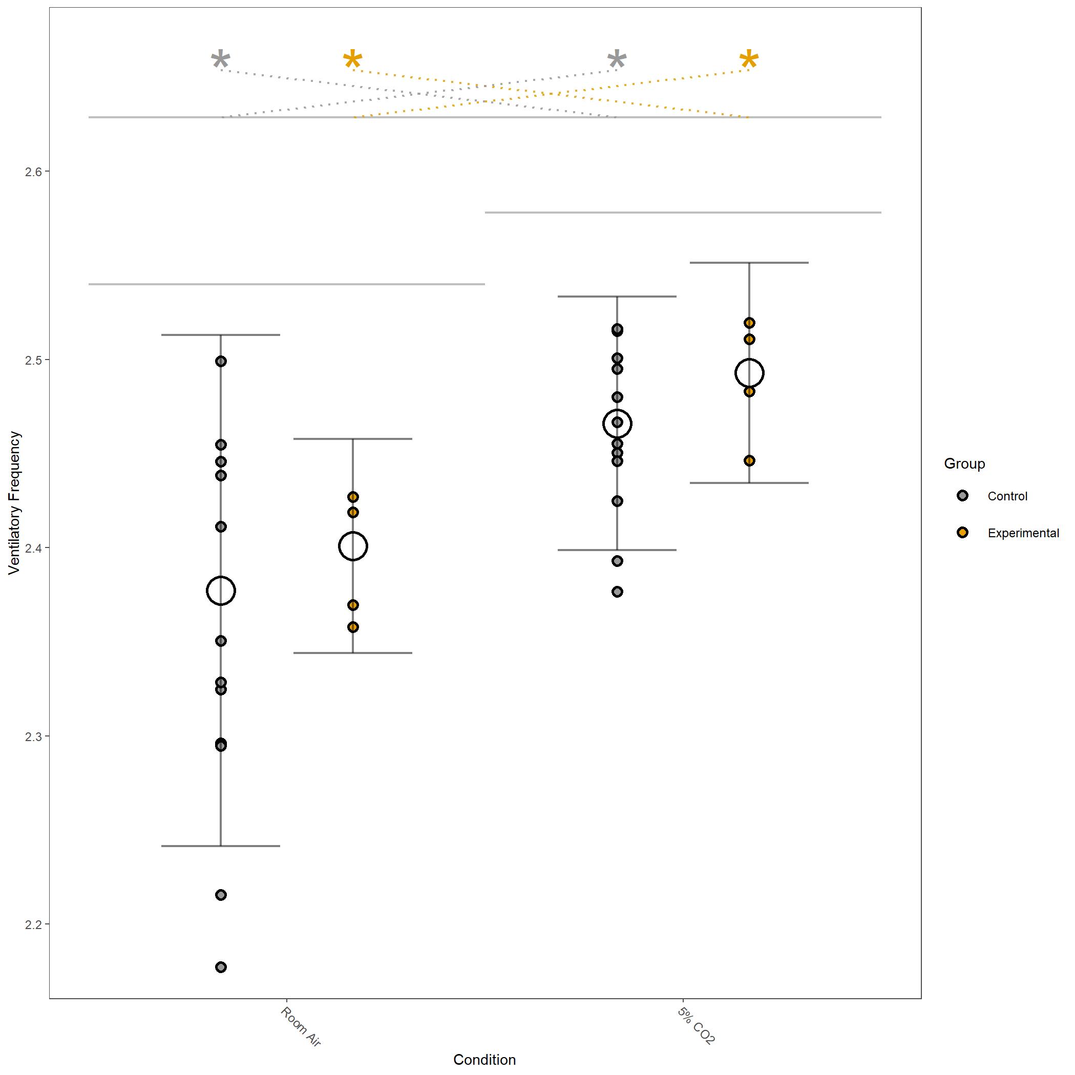
Log10 transformed Ventilatory Frequency for vignette dataset.
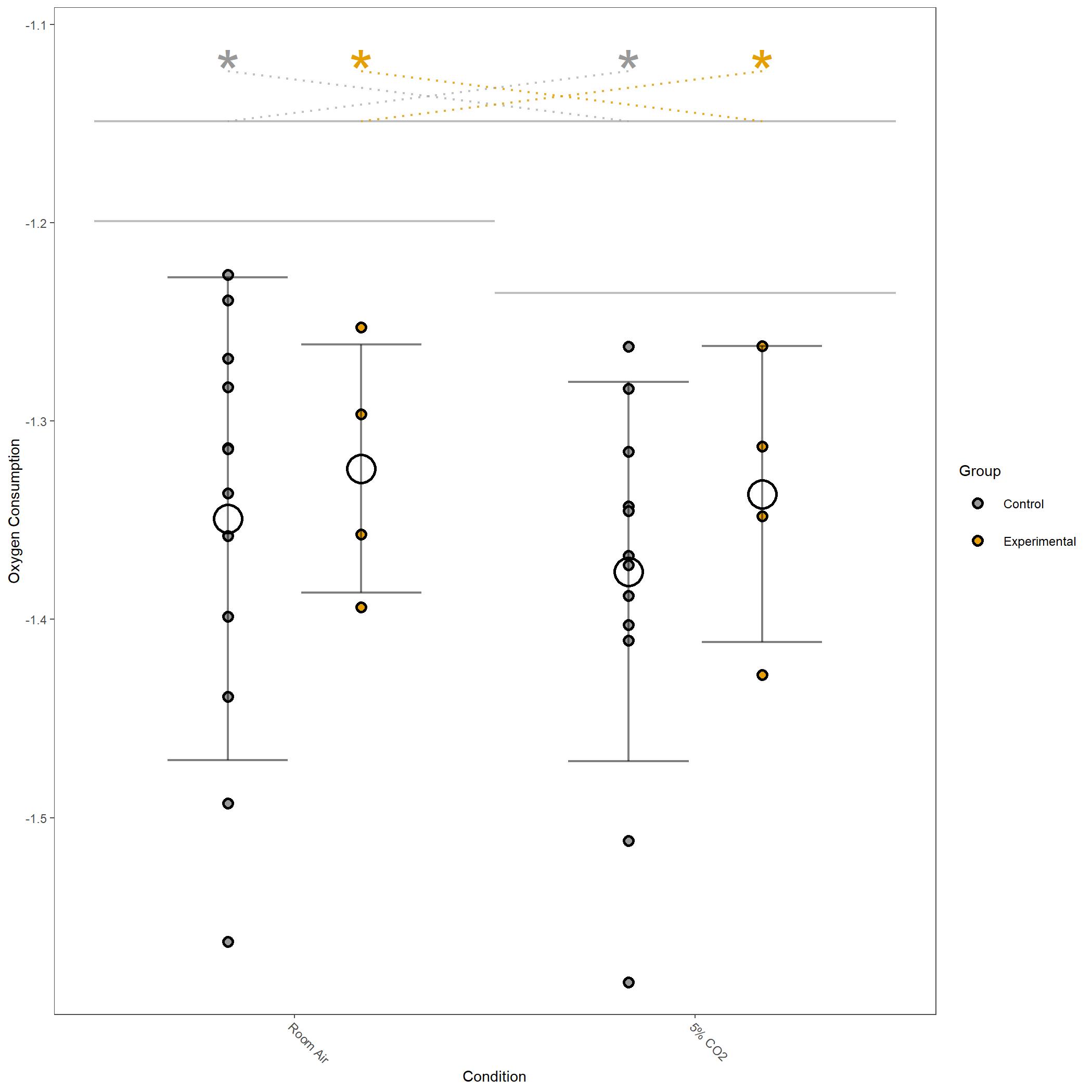
Log10 transformed Oxygen Consumption for vignette dataset.
For this run we have also produced poincare plots for the respiratory variables plotted. Here we show poincare plots for Breath Cycle Duration for room air and 5% CO2 to show the difference in distribution of BCD values. You can appreciate that there is shift to have longer breath cycles during 5% CO2 compared to room air. You can also see that the duration of breaths are much more consistent in 5% CO2 compared to room air, which is expected.
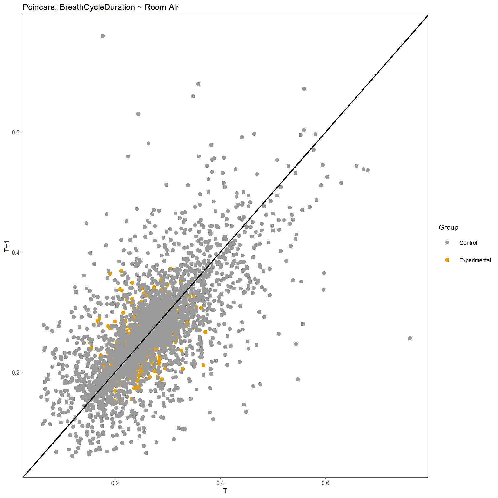
Poincare plot of Breath Cycle Duration for all breaths included during room air for this dataset.
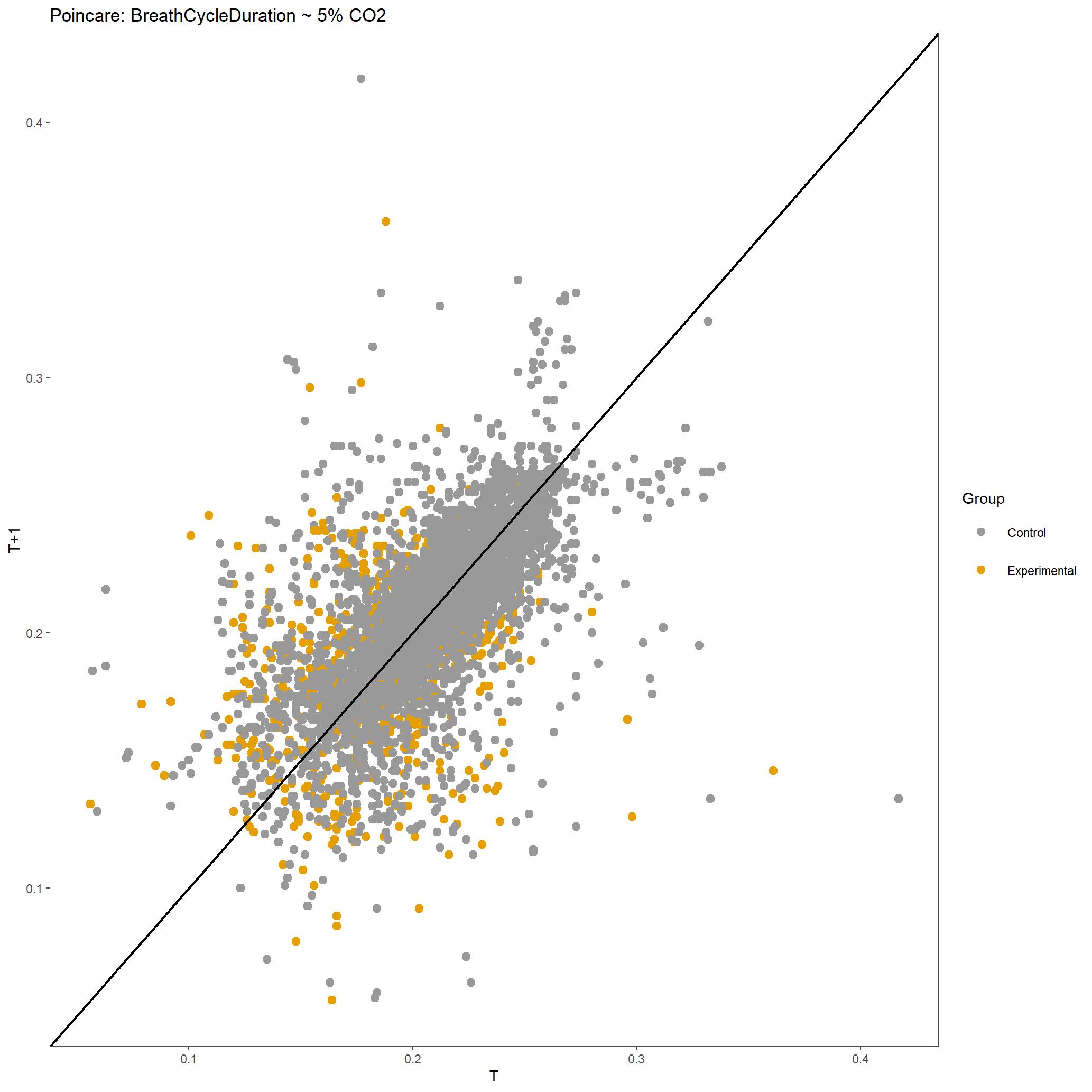
Poincare plot of Breath Cycle Duration for all breaths included during 5% CO2 for this dataset.
Within the StatResults folder are the residual and QQ plots for all transformations. These are used to determine
the most appropriate transformation for each variable. To demonstrate the use of these, we’ve hightlight the selection
of the appropriate transformation of Ventilation below where the raw values, log10 transformed, and
square root transformed QQ and residual plots are shown. We chose square root transformed becuase the QQ plot showed the most
linear-like distribution and the residual plot was least skewed for that transformation of the data. This is the process
that was completed for each of the variables above to select the appropriate statistical outcomes.
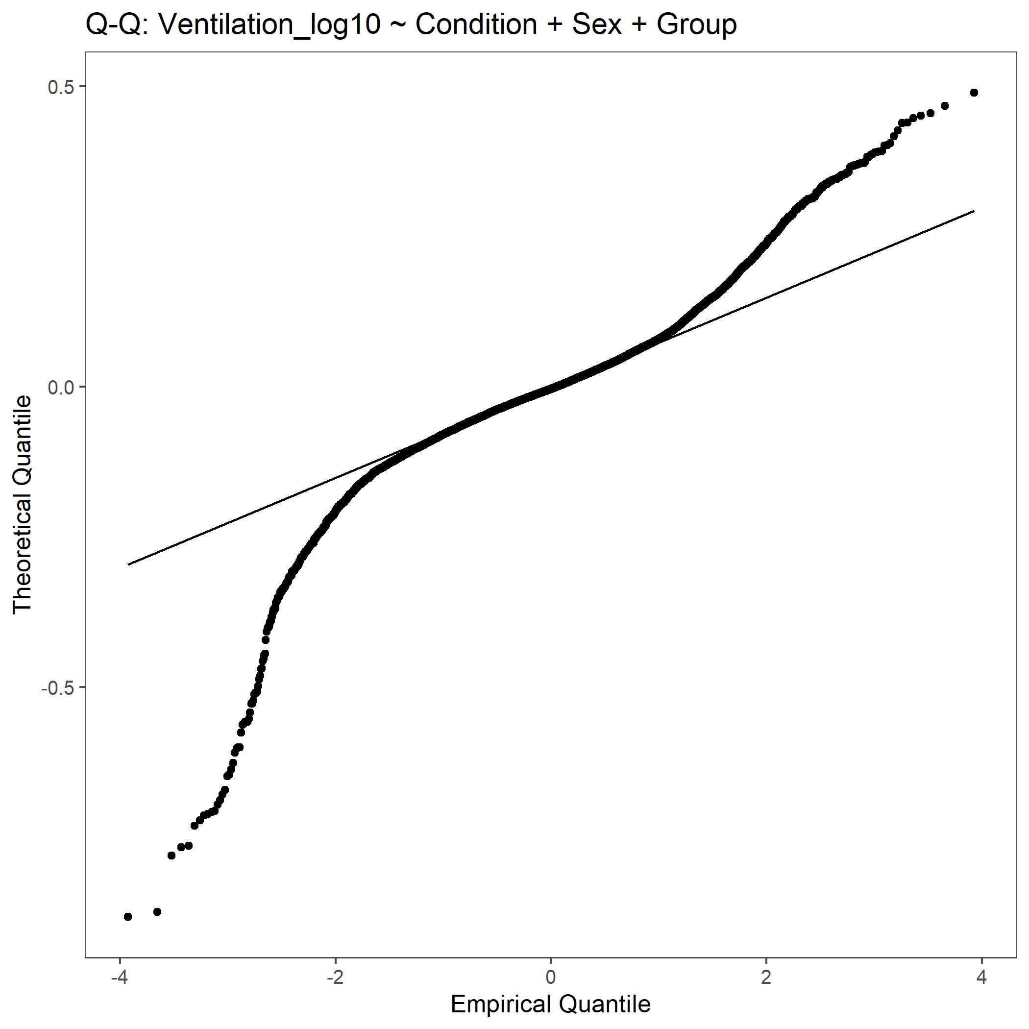
QQ plot for Ventilation with log10 transformed data.
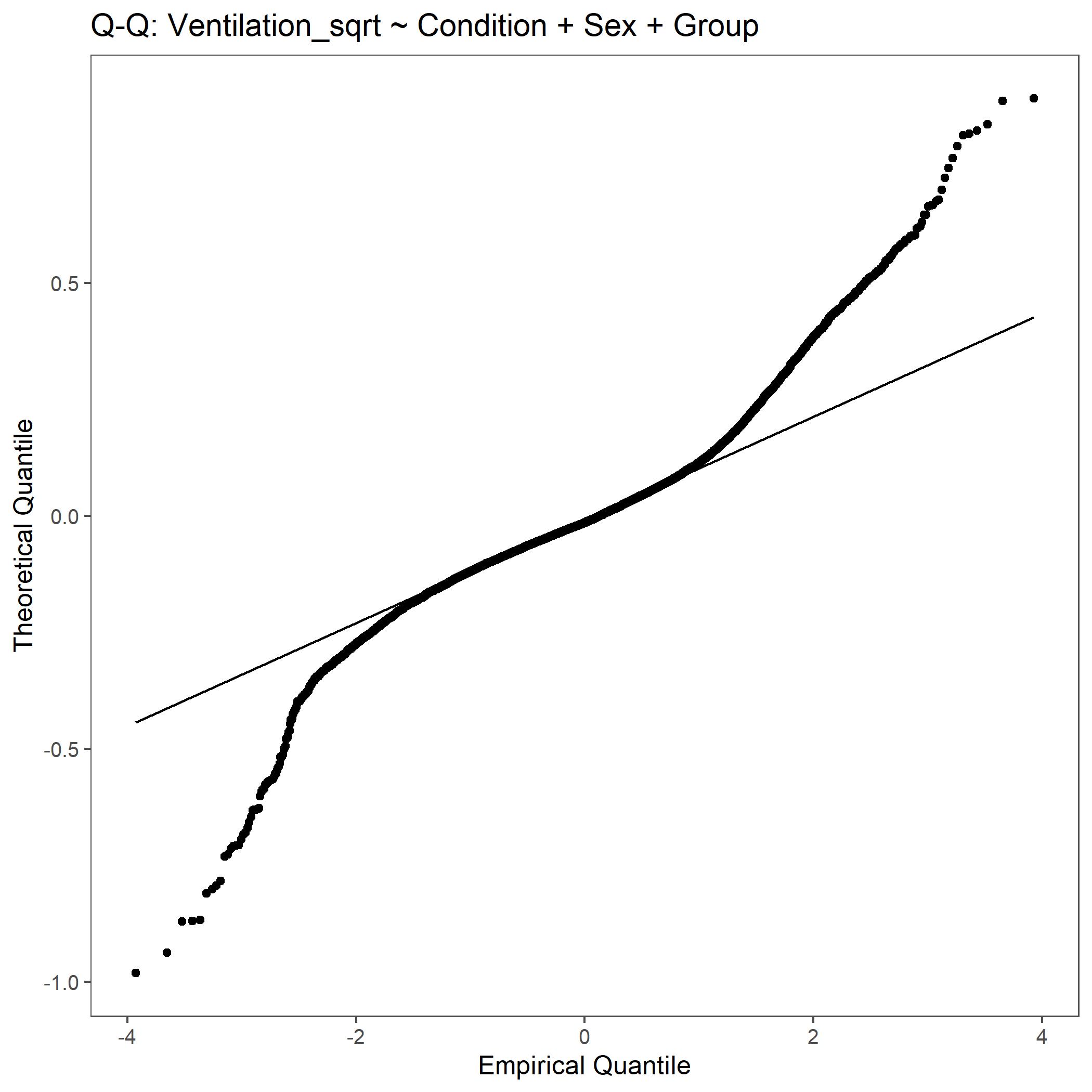
QQ plot for Ventilation with square root transformed data.
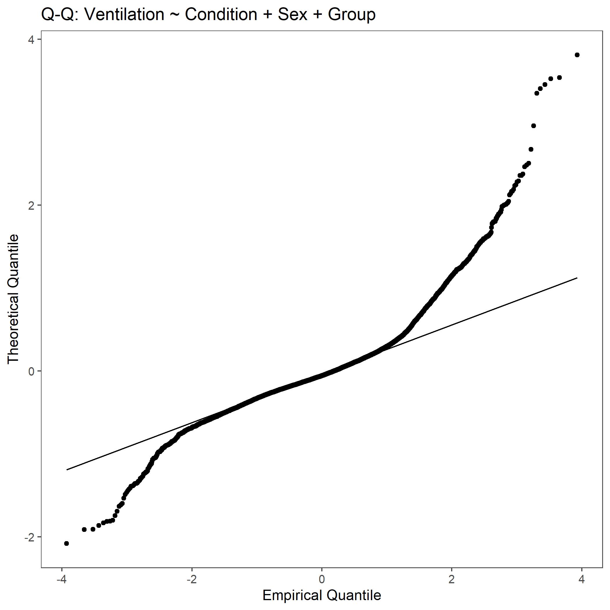
QQ plot for Ventilation with non-transformed, raw data.
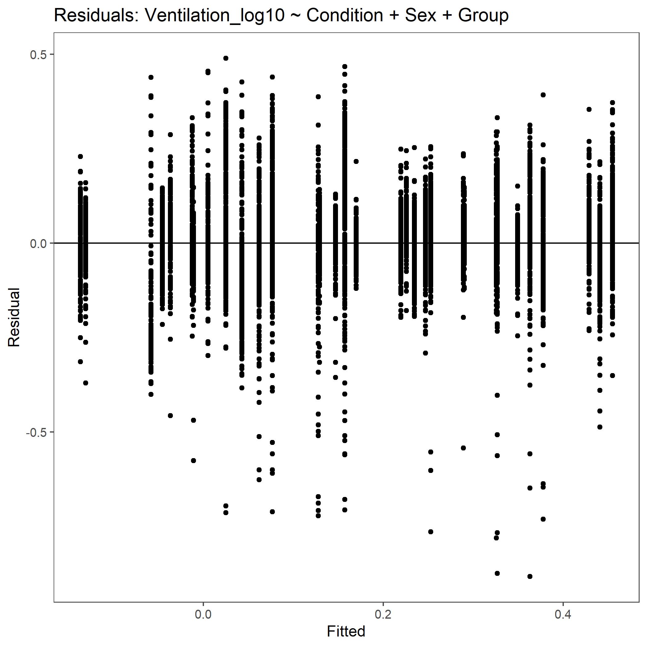
Residual plot for Ventilation with log10 transformed data.
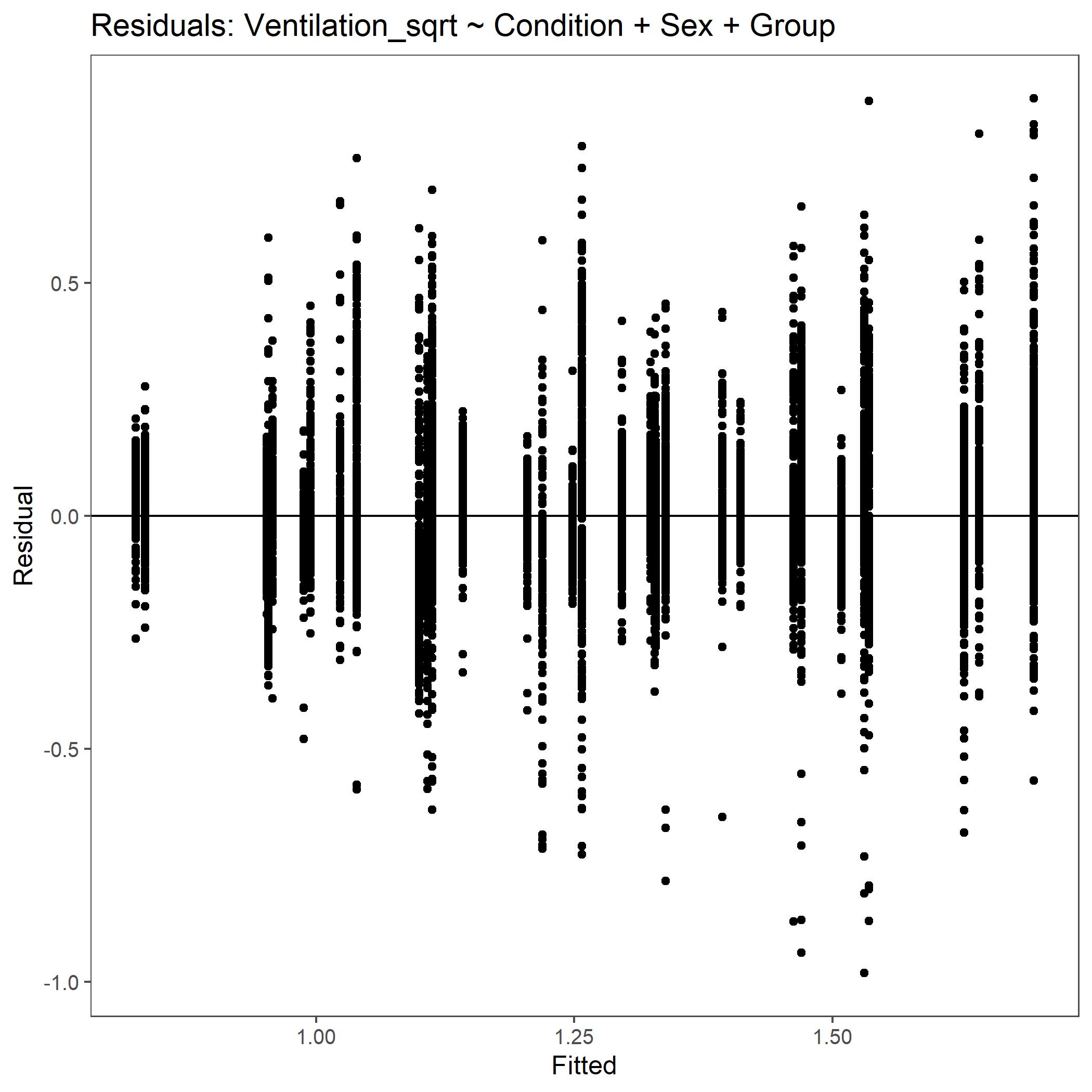
Residual plot for Ventilation with square root transformed data.
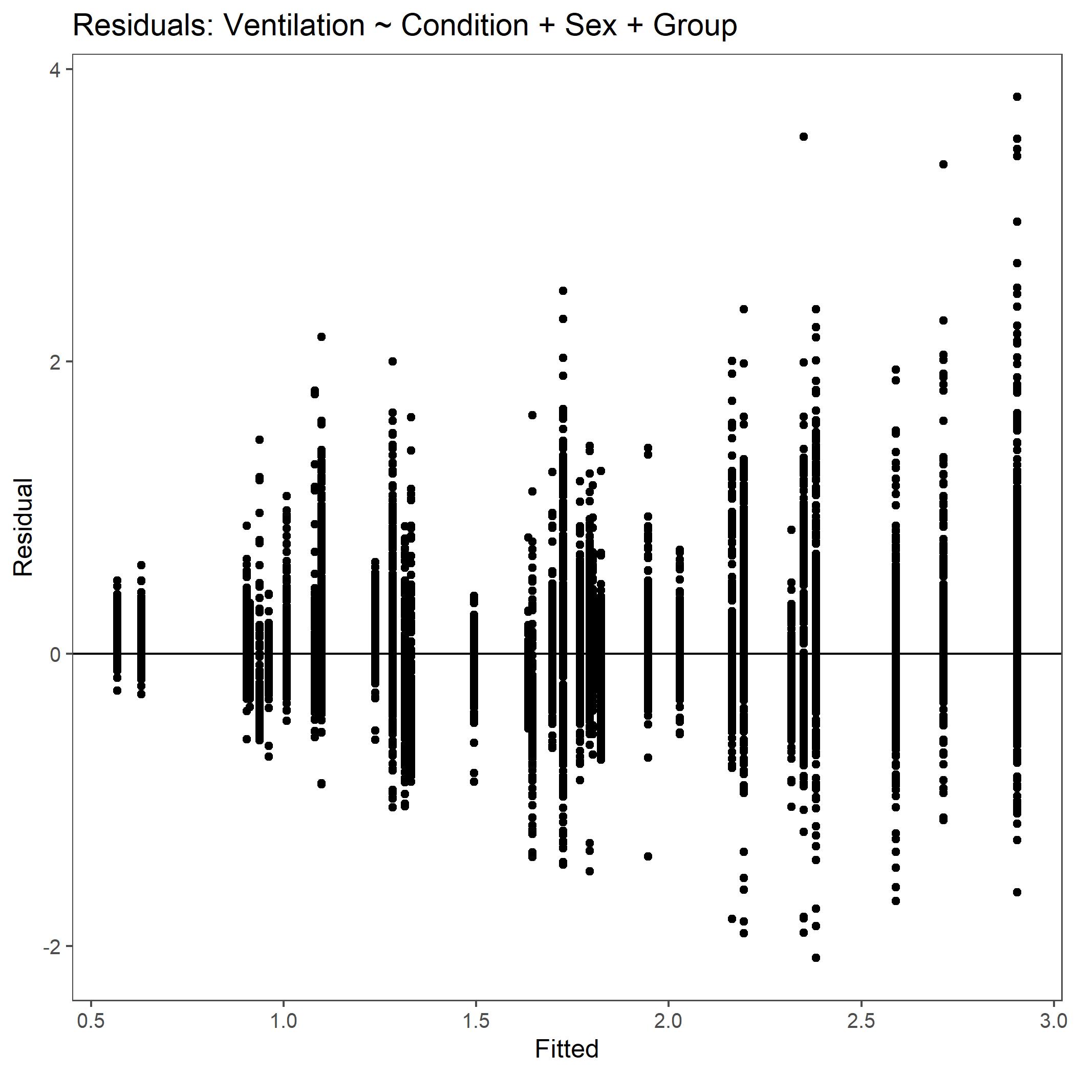
Residual plot for Ventilation with non-transformed, raw data.